
Analyzing Data
Staff Directory
Introduction
Simply put, analyzing data is the process of turning raw data or information into a meaningful summary or set of methodically derived inferences. Analyzing data is a critical component of the three investigative approaches mentioned in Module 10: assessment, “improvement and accountability”, evaluation, “judgement against a standard”, and research, “to produce generalizable knowledge.” It is important to recognize, though, that analyzing data does not take place in a vacuum. As graphically depicted in the Assessment Cycle diagram in Module 3, there are a number of steps leading up to data analysis and all decisions that are made (or not made) in those steps directly impact our opportunities and limitations for analyzing data or information. For example, if an investigator would like to perform a thematic analysis of qualitative response data, it is important that the data collection tool (i.e., survey) is designed to effectively capture response data with themes that align with the purpose or goal of the investigation, which is the first step in the Assessment Cycle.
Overview
To ensure best practices for data analysis, it is essential for the investigator to begin by answering a few questions.
Context: Before diving in to analyze/interpret data, consider, what has been done in the previous stages of the Assessment Cycle (Module 3)? This review of what has or has not been completed leading up to the process of analyzing data will inform what analytical options are at the investigator’s disposal.
Variable Level: What type(s) of data do will be used in the analysis? Beyond determining if the data is qualitative or quantitative, the general characteristics of data are based on the type of measurement scale.
Goals: What are the analysis goals? These should be aligned with, and a natural extension of, the earlier Purpose and Determine Methodology stages of the Assessment Cycle. Potential data analysis goals include:
• Reporting – Providing a quick summary of results or themes (Module 8)
• Exploration – Investigating data for connections or themes, motivated by curiosity rather than a clear goal
• Research – “diligent and systematic inquiry or investigation into a subject in order to discover or revise facts, theories, applications, etc.” (Dictionary.com, n.d.).
Considerations for Analyzing Data
Data Collection – the process of methodically gathering information for the likely eventual purpose of data analysis.
• Focus group and interview (Module 6)
• Document review
• Survey and questionnaire (Module 5)
• Observation
• Experiments
*Note: The data collection methods above may be used to support qualitative or quantitative data analyses and are simply dependent upon the type of data or variable level collected.
Data Cleaning – “Data cleaning is an overloaded term and is often used loosely to refer to a variety of tasks aimed at improving the quality of data” (Ganti & Sarma, 2013).
Common tasks of data cleaning:
• Data Standardization: ensuring that all attribute values keep the same data format and content. For example, the variable ID requires the data to be string type and has 8 digits. Date should be YYYYMMDD format and gender requires to be a single cap letter.
Table 1
| ID | Date | Gender |
|---|---|---|
| 56457 | 20200827 | F |
| 6579546 | 8/27/2020 | female |
| 13548952 | 8/27/2020 | f |
Table 2
| ID | Date | Gender |
|---|---|---|
| 00056457 | 20200827 | F |
| 06579546 | 20200827 | F |
| 13548952 | 20200827 | F |
• Data Profiling: The process of evaluating data quality. For example, one may expect the customer name and address columns uniquely determine each customer record in a Customer relation. In such a case, the number of unique [name, address] values must be close to that of the total number of records in the Customer relation (Ganti & Sarma, 2013).
• Deduplication: The goal of deduplication is to group records in a table such that each group of records represents the same entity. Table 3 showing records with {g11, g12, g13} being one group of duplications, and {g21, g22} another set of duplicate records. And we can combine the group g11, g12, and g13 to obtain a single record t as indicated by Table 4 (Ganti & Sarma, 2013).
Table 3
| ID | Name | Country |
|---|---|---|
| g11 | Roger Federrer | Switzerland |
| g12 | R. Federer | Switzerland |
| g13 | Roger Federer | Swiss |
| g21 | Novak Djokovic | Serbia |
| g22 | Novak Jokavic | Serbia |
Table 4
| ID | Name | Country |
|---|---|---|
| t | Roger Federer | Switzerland |
• Record Matching: The goal of record matching is to match each record from a set of records with records in another table. Consider a scenario when a new batch of customer records is being imported into a sales database. In this scenario, it is important to verify whether the same customer is represented in both the existing as well as the incoming sets and only retain one record in the final result. Due to representational differences and errors, records in both batches could be different and may not match exactly on their key attributes (e.g., name and address or the CustomerId). The goal of a record matching task is to identify record pairs, one in each of two input relations, which correspond to the same real-world entity (Ganti & Sarma, 2013).
Table 5
| ID | Name | Street | City | Phone |
|---|---|---|---|---|
| r1 | Sweetlegal Investments Inc | 202 North | Redmond | 425-444-5555 |
| r2 | ABC Groceries Corp | Amphitheatre PKwy | Mountain View | 4081112222 |
| r3 | Cable Television Services | One Oxford Dr | Cambridge | 617-123-4567 |
| s1 | Sweet legal Investments Incorporated | 202 N | Redmond | |
| s2 | ABC Groceries Corpn. | Amphitheetre Parkway | Mountain View | |
| s3 | Cable Services | One Oxford Dr | Cambridge | 6171234567 |
• Schema Matching: To align attributes from different schemas. For example, suppose the information from our warehouse example was organized as a relation R (Name, City Address, Country, Phone). Now suppose you obtain another relation with data represented in the format S (Company, Street, City, Zip, Nation, Phone number). To populate records from S into R, we need a process to convert each S record into the format of R. Schema matching provides: (1) attribute correspondences describing which attributes in S correspond to attributes in R; e.g., Country corresponds to Nation, Phone, Number corresponds to Phone, Company corresponds to Name, and City Address corresponds to the remaining four attributes in S (2) transformation functions give concrete functions to obtain attribute values in R from attribute values in S; e.g., a transformation process gives a mechanism to concatenate all attributes to form City Address (or extract attributes like Zip code when converting R to S) (Ganti & Sarma, 2013).
Relation R
| Name | Address | Country | Phone |
|---|---|---|---|
| Company1 | 1358 Museum Rd, Gainesville, FL 32603 | USA | 123-456-789 |
Relation S
| Company | Street | City | State | Zip | Nation | Phone Number |
|---|---|---|---|---|---|---|
| Company2 | 3100 Museum Rd | Gainesville | FL | 32611 | USA | 66-789-123 |
Analysis Methodologies
Qualitative: Qualitative analysis is the process of examining and utilizing manualized procedures on non-numeric data to elicit condensed forms that reveal key takeaways and conclusions related to the experiences, opinions and/or phenomenologies of participants.
There are many different types of qualitative methodologies, such as thematic analysis, phenomenology, narratives, ethnography, case studies, and grounded theory (Henning & Roberts, 2016). In general, however, each is based in a similar procedure. The data (interview and/or focus group transcripts) are reviewed and significant quotes are identified. These quotes are sorted into “themes” identified by the researcher (often according to theory). After reviewing the data a few times, resultant themes must then be organized and trimmed to create a narrative of quotes that summarize the key points across all of the data.
Qualitative analysis can be completed without the use of specialized software; often it is sufficient to rely on word processing programs to copy/paste quotes and develop themes. However, this process can be made easier with programs such as NVivo. Thematic analysis is one of the more straightforward forms of qualitative analysis, with more lenient participation requirements. The following article provides a step-by-step manual for completing this methodology.
https://www.researchgate.net/publication/235356393_Using_thematic_analysis_in_psychology (Braun & Clarke, 2006).
Quantitative: that relies primarily on the collection of quantitative data (Johnson & Christensen, 2010)
Table 6 - Levels of Measurement
| Variable Types | Definition | Example | |
|---|---|---|---|
| Categorical | Nominal | Essentially “labels,” without quantitative value or overlap | major, degree type, or residence hall could all be assessed as nominal data |
| Dichotomous | Only has two levels or variables | yes/no, present/absent, pass/fail | |
| Ordinal | Data that are non-numeric concepts that are organized in a specific order, such as level of satisfaction or agreement | Descriptive scales such as, “Unsatisfied”, “Slightly unsatisfied”, “Neither satisfied nor unsatisfied”, “Slightly satisfied”, “Satisfied” | |
| Quantitative | Discrete | Counts of individual items or values | Number of students in a class, Number of different tree species in a forest |
| Continuous | Measurements of continuous or non-finite values. | Distance, Volume, Age | |
Table 7 - Additional Common Variables
| Additional Common Variables | Definition | Example |
|---|---|---|
| Independent variable | A variable that is presumed to cause changes to occur in another variable; a causal variable | Amount of Studying (IV) affects test grades (DV) |
| Dependent variable | A variable changes because of another variable; the effect or outcome variable | Amount of Studying (IV) affects test grades (DV) |
| Mediating variable | A variable that comes in between other variable, helping to delineate the process through which variable affect one another | Amount of Studying (IV) leads to input and organization of knowledge in long-term memory (mediating variable), which affects test grades (DV) |
| Moderator variable | A variable that delineated how a relationship of interest changes under different condition or circumstance | Perhaps the relationship between studying (IV) and test grade (DV) changes according to the different level of use of a drug such as Ritalin (moderator) |
| Extraneous variable | A variable that may compete with the independent variable in explaining an outcome | Perhaps the relationship between Coffee drinking (IV) and cancer (DV) is actually due to smoking. |
Experimental Research: Determine cause-and-effect relationships. The experimental research method enables us to identify causal relationships because it allows us to observe, under controlled conditions, the effects of systematically changing one or more variables (Johnson & Christensen, 2010).
Nonexperimental Research: Research in which the independent variable is not manipulated and there is no random assignment to groups (Johnson & Christensen, 2010).
• Correlational studies describe the relative nature and strength of one variable’s relation (or lack of relation) to another variable without the experimental manipulation of one or more variables (Heiman, 2003).
• Correlation coefficient: A numerical index that indicates the strength and direction of the relationship between two variables (Johnson & Christensen, 2010).
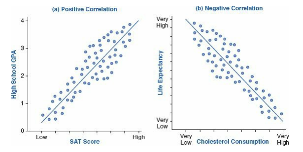
• Positive correlation: The situation when scores on two variables tend to move in the same direction (Johnson & Christensen, 2010).
• Negative correlation: The situation when scores on two variables tend to move in opposite directions (Johnson & Christensen, 2010).
Table 8 – Examples of positive and negative correlation
Data Mining is “the automated or convenient extraction of patterns representing knowledge implicitly stored or captured in large databases, data warehouses, the web, other massive information repositories, or data streams” (Han, Pei & Kamber, 2012, p. xxiii).
Mixed Method: Research that involves the mixing of quantitative and qualitative methods or other paradigm characteristics (Johnson & Christensen, 2010).
Statistics
The practice or science of collecting and analyzing numerical data in large quantities, especially for the purpose of inferring proportions from those in a representative sample (lexico, n.d.).
Descriptive Statistics: Statistics that focus on describing, summarizing, or explaining data. Although the results from this type of analysis can be useful for drawing general conclusions about the data set as a whole, it is not possible to make conclusions regarding the total population. Examples of descriptive statistics include measures of central tendency (mean, median, and mode) and measures of spread (e.g., variance and standard deviation), as well as measures of kurtosis and skewness (Toward Data Science, n.d.).
Using Microsoft Excel, it is relatively easy to calculate a data set’s descriptive statistics using an Excel plugin (excel-easy.com, n.d.) or by using formulas for specific statistics such as average, median, mode, and standard deviation (Exceljet.com, n.d.).
Inferential Statistics: Statistics that go beyond the immediate data and infer the characteristics of populations based on samples (Johnson & Christensen, 2010).
• Regression Analysis: is a set of statistical procedures used to explain or predict the values of a dependent variable based on the values of one or more independent variables (Johnson & Christensen, 2010).
o Simple regression: Regression based on one dependent variable and one independent variable (Johnson & Christensen, 2010).
• Here is the simple regression equation formula: Ŷ = a + bX
• where (Ŷ called Y-hat) is the predicted value of the dependent variable, a is the y-intercept(The point where the regression line crosses the y-axis ), b is the regression coefficient (The predicted change in Y given a 1-unit change in X), and X is the single independent variable.
Here is the simple regression equation formula: Ŷ = a + bX
o Multiple regression: Regression based on one dependent variable and two or more independent variables (Johnson & Christensen, 2010).
• Hypothesis testing: evaluates two mutually exclusive statements about a population to determine which statement is best supported by the sample data (Towards Data Science, n.d.).
o Null Hypothesis (H₀) – A statement in which no difference or effect is expected. If the null hypothesis is not rejected, no changes will be made (Towards Data Science, n.d.).
o Alternate Hypothesis (H₁) – A statement that some difference or effect is expected. Accepting the alternative hypothesis will lead to changes in opinions or actions. It is the opposite of the null hypothesis (Towards Data Science, n.d.).
Table 9 – Example of Null and Alternate Hypothesis in inferential statistics
| Research Question | Null Hypothesis | Symbolic H₀ Hypothesis | Alternate Hypothesis | Symbolic H₁ Hypothesis |
|---|---|---|---|---|
| Do teachers score higher on the GRE Verbal than the national average? | The teacher population GRE Verbal mean is equal to the national average of 476 | H₀ :µGRE=476 | The Teacher population GRE Verbal mean is different from the national average of 476 | H₁ :µGRE ≠ 476 |
| Do male or females tend to score better on the GRE Verbal? | The male and female population means are not different | H₀ :µM=µF | The male and female population means are not different | H₁ :µm≠ µF |
| Do education, arts and sciences and business students have different starting income? | The Education, arts and sciences and business students population have the same mean starting income | H₀ :µE=µA=µB | The Education, arts and sciences and business students population have the same mean starting income | H₁ :Not all equal |
| Is there a correlation between GPA(X) and starting salary | The population correlation between GPA and starting salary is equal to zero. | H₀ :ρXY =0 | The population correlation between GPA and starting salary is NOT equal to zero. | H₁ :ρXY ≠0 |
| Is there a relationship between GRE Verbal(X1) and starting salary (Y), Controlling for GPA(X2) | The population regression coefficient is equal to zero. | H₀ :βYx1,x2 =0 | The population regression coefficient is not equal to zero. | H₁: βYx1,x2 ≠0 |
(Johnson & Christensen, 2010)
- T test for independent samples: Statistical test used to determine whether the difference between the means of two groups is statistically significant.
- One-way ANOVA: Statistical test used to compare two or more group means.
- Chi-Square Test: The Chi-square test of independence (also known as the Pearson Chi-square test, or simply the Chi-square) is one of the most useful statistics for testing hypotheses when the variables are nominal (McHugh, 2013).
Statistical Analysis Test Selection: Using the steps above, the key ingredients to selecting the appropriate statistical test are
1. Variable level
2. Total independent variables and dependent variables
3. Distribution of data (normally distributed) and sample size
4. Goal of analysis
*Note: Statistical test decision trees are excellent tools for determining which test to use. See below for a great (but by no means the only) example.
Table 10 – Statistical Analysis Test Selection

(Tronstad, 2014)